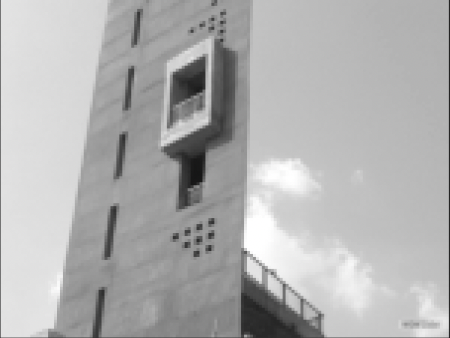
Edge Detection
Edge Detection in Images using OpenCV and Python.
GitHub Repository
Keywords
Fourier Series,Convolution,Discrete Fourier Transform Fast Fourier Transform, Inverse Fourier Transform,Windowing,Zero Padding,Numpy,Matplotlib,OpenCV.
Algorithm
1. Image Representation: We define the image as a 2-d function f(x,y) where x and y are spatial coordinates and the amplitude of f at any pair of coordinates (x,y) and the intensity values of the image at that point. For a sinusoidal signal, if the amplitude varies so fast in a short time, you can say it is a high frequency signal. Edges are significant local changes of intensity in an image. More intuitively, at edges the amplitude varies drastically in images. So we can say, edges are high frequency content in images.
# Importing numpy, cv2 and matplotlib

import cv2 as cv
import numpy as np
from matplotlib import pyplot as plt

# Reading image in grayscale
img = cv.imread('lal_minar.jpg', 0)

# Frequency transform is a complex array
f = np.fft.fft2(img)

# Shifting the zero frequency component to the center
fshift = np.fft.fftshift(f)

# Finding the magnitude spectrum
A1 = 20
magnitude_spectrum = A1 * np.log(np.abs(fshift))

# Plotting
plt.subplot(121), plt.imshow(img, cmap='gray')
plt.title('Input Image'), plt.xticks([]), plt.yticks([])
plt.subplot(122), plt.imshow(magnitude_spectrum, cmap='gray')
plt.title('Magnitude Spectrum'), plt.xticks([]), plt.yticks([])
plt.show()

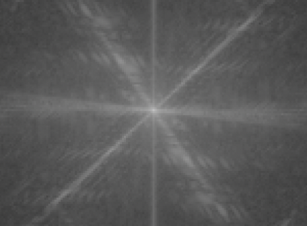
2. Understanding Frequency Components and Edges: Once we perform the fourier transform of an image, we would see a plot of high and low frequencies. Interestingly, all the low frequency components are saturated at the center, and the high frequency components are scattered around. We then create a high pass filter which would typically be a mask array of the same size as the image with a miniature square of zeroes at the center and rest all ones.
# Center
rows, cols = img.shape
crow, ccol = rows // 2, cols // 2

# HPF masking, center 12X12 grid masked 0, remaining all ones
mask = 12
fshift[crow - mask:crow + mask, ccol - mask:ccol + mask] = 0

# Finding the magnitude spectrum of masked Fourier Transform
A2 = 2000
fshift_mask_mag = A2 * np.log(np.abs(fshift))

# Plotting
plt.imshow(fshift_mask_mag, cmap='gray')
plt.title('FFT + Mask'), plt.xticks([]), plt.yticks([])
plt.show()
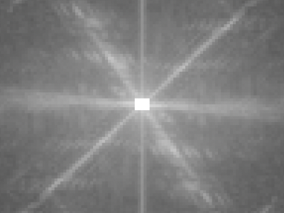
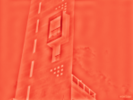
3. Image Restoration and Inverse Fourier Transform: Now when the mask is applied to the original image, the resultant would only have high frequencies. This becomes quite useful as low frequencies correspond to non-edges in the spatial domain. The result shows High Pass Filtering is an edge detection operation.
# Restoring the original indexing
f_ishift = np.fft.ifftshift(fshift)

# Inverse FFT
img_back = np.fft.ifft2(f_ishift)

# Finding the magnitude spectrum
img_back = np.real(img_back)

# Plotting
plt.subplot(121), plt.imshow(img, cmap='gray')
plt.title('Lal Minar'), plt.xticks([]), plt.yticks([])
plt.subplot(122), plt.imshow(img_back, cmap='Reds')
plt.title('Image after HPF'), plt.xticks([]), plt.yticks([])
plt.show()
